Week 6A: Area under a function

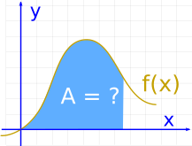
Is the area under a curve a topic of single variable calculus? Image by mathisfun.com

Consider the Cartesian x−yx-y plane. The area AA of some surface (Γ\Gamma) may be computed as integral of infinitely small surface elements dA=dxdy\mathrm{d}A = \mathrm{d}x\mathrm{d}y,

A=∬ΓdxdyA = \iint_{\Gamma}\mathrm{d}x\mathrm{dy}

Lets say we want to compute the surface area of the blue-shaded area in the figure. This area is bound by the function y=f(x)>0y = f(x) > 0 and y=0y = 0 for x∈⟨a,b⟩x \in \langle a, b\rangle. We can write

A=∬Γdydx=∫ab∫0f(x)dydxA = \iint_{\Gamma}\mathrm{dy}\mathrm{d}x = \int_{a}^{b}\int_0^{f(x)}\mathrm{d}y\mathrm{d}x =∫abf(x)dx.= \int_{a}^{b}f(x)\mathrm{d}x.

This results corresponds to what you already knew from your single-variable Calculus course.

Thank you multiple integration! for degenerating into single-variable calculus in this limit.

Week 6B: Work done by a force field

Consider a particle moving in a circular trajectory with radius RR, angular frequency ω\omega, and time parameter tt,

r⃗(t)=Rcos(ωt)e⃗x+Rsin(ωt)e⃗y.\vec{r}(t) = R\cos(\omega t)\vec{e}_x + R\sin(\omega t)\vec{e}_y.

It is affected by a force field (F⃗(x,y)\vec{F}(x,y)) given by,

F⃗(x,y)=−ye⃗x.\vec{F}(x,y) = -y\vec{e}_x.

We can compute the work (WW) done on this particle during a single rotation as the line integral of infinitely small work sections dW=F⃗⋅dr⃗\mathrm{d}W = \vec{F}\cdot\mathrm{d}\vec{r}. Because we know we want to integrate force over a distance, it would be nice if we could integrate over the displaced (from 0 to 2πR2\pi R). As such we look for the paramterization in terms of its intrinsic parameter (i.e. path length). For this simple paramterization, we can rewrite the coordinate r⃗\vec{r} as a function of time into a function of the traveled distance (ss), such that ∥dr⃗ds∥=1\| \frac{\mathrm{d}\vec{r}}{\mathrm{d}s}\| = 1. Fortunately there is a simple invertible relation s(t)s(t),

s(t)=∫0t∥dr⃗(τ)dτ∥dτ=[R2ω2sin2(ωτ)+R2ω2cos2(ωτ)]0t=[Rωsin2(ωτ)+cos2(ωτ)]0t=Rω[1]0t=Rωt.\begin{align} s(t) &= \int_0^{t} \|\frac{\mathrm{d}\vec{r}(\tau)}{\mathrm{d}\tau}\| \mathrm{d}\tau \\ &= \left[ \sqrt{R^2\omega^2\sin^2 (\omega \tau) + R^2\omega^2\cos^2 (\omega \tau)}\right]_0^t\\ &= \left[R\omega \sqrt{\sin^2 (\omega \tau) +\cos^2 (\omega \tau)}\right]_0^t\\ &= R\omega [1]_0^t = R\omega t. \end{align}

and its inverse,

t(s)=sRω.t(s) = \frac{s}{R\omega}.

Such that

r⃗(s)=Rcos(sR)e⃗x+Rsin(sR)e⃗y.\vec{r}(s) = R\cos(\frac{s}{R})\vec{e}_x + R\sin(\frac{s}{R})\vec{e}_y.

So for the work we may write,

W=∫F⃗⋅dr⃗=∫02πRF⃗⋅t⃗ds.W = \int \vec{F}\cdot \mathrm{d}\vec{r} = \int_0^{2\pi R} \vec{F}\cdot \vec{t}\mathrm{d}s.

With t⃗\vec{t} the (unit) tangential vector and not to be confused with the time parameter (tt),

t⃗=dr⃗(s)ds=−sin(sR)e⃗x+cos(sR)e⃗y.\vec{t} = \frac{\mathrm{d}\vec{r}(s)}{\mathrm{d}s} = -\sin(\frac{s}{R})\vec{e}_x + \cos(\frac{s}{R})\vec{e}_y.

Such that the inner product

F⃗⋅t⃗=ysin(sR),\vec{F}\cdot\vec{t} = y\sin(\frac{s}{R}),

We know from the parameterization y(s)=Rsin(sR)y(s) = R\sin(\frac{s}{R}). Thus,

F⃗⋅t⃗=Rsin2(sR).\vec{F}\cdot\vec{t} = R\sin^2(\frac{s}{R}).

Resulting in the integral,

W=∫02πRF⃗⋅t⃗ds=R∫02πRsin2(sR)ds.=R∫02πR12(1−cos(2sR))ds.=R2[s−R2sin(2sR)]02πRds=πR2.\begin{align} W &= \int_0^{2\pi R} \vec{F}\cdot \vec{t}\mathrm{d}s = R\int_0^{2\pi R} \sin^2(\frac{s}{R}) \mathrm{d}s.\\ &= R\int_0^{2\pi R} \frac{1}{2}\left( 1-\cos(\frac{2s}{R}) \right)\mathrm{d}s.\\ &= \frac{R}{2} \left[ s - \frac{R}{2}\sin(\frac{2s}{R}) \right]_0^{2\pi R} \mathrm{d}s\\ &= \pi R^2. \end{align}

Thank you line integral, I guess. But isn’t there an easier way?

Continue to the examples of week 7…

The marvelous design of this website is taken from Suckless.org